This article follows up on the series devoted to k-means clustering at The Data Science Lab. Previous posts have dealt with how to implement Lloyd’s algorithm for clustering in python, described an improved initialization algorithm for proper seeding of the initial clusters, k-means++, and introduced the gap statistic as a method of finding the optimal K for k-means clustering.
Although the gap statistic, based on a paper by Tibshirani et al was shown to find optimal values for the number of clusters in a variety of cases when the clusters where globular and mildly disjointed, its performance might be hampered by the need of perfoming Monte Carlo simulations to estimate the reference datasets. A reader of this blog, Jonathan Stray, pointed out a potentially superior method for selecting the K in k-means clustering, so let us implement it and compare.
An alternative approach to finding the optimal K
The approach suggested by our reader is based on a publication by Pham, Dimov and Nguyen from 2004. The article is very much worth reading, as it includes an explanation of the drawbacks of the standard k-means algorithm as well as a comprehensive survey on different methods that have been proposed for selecting an optimal number of clusters.
In section 3 of the paper, the authors justify the introduction of a function  to evaluate the quality of the resulting clustering and help decide on the optimal value of
  for each data set. Quoting from the paper:
A data set with  objects could be grouped into any number of clusters between 1 and , which would correspond to the lowest and the highest levels of detail respectively. By specifying different values, it is possible to assess the results of grouping objects into various numbers of clusters. From this evaluation, more than one value could be recommended to users, but the final selection is made by them.
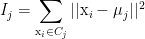
The goal of a clustering algorithm is to identify regions in which the data points are concentrated. It is also important to analyze the internal distribution of each cluster as well as its relation to other clusters in the data set. The distorsion of a cluster is a measure of the distance between points in a cluster and its centroid:
 .
.
The global impact of all clusters’ distortions is given by the quantity
 .
.
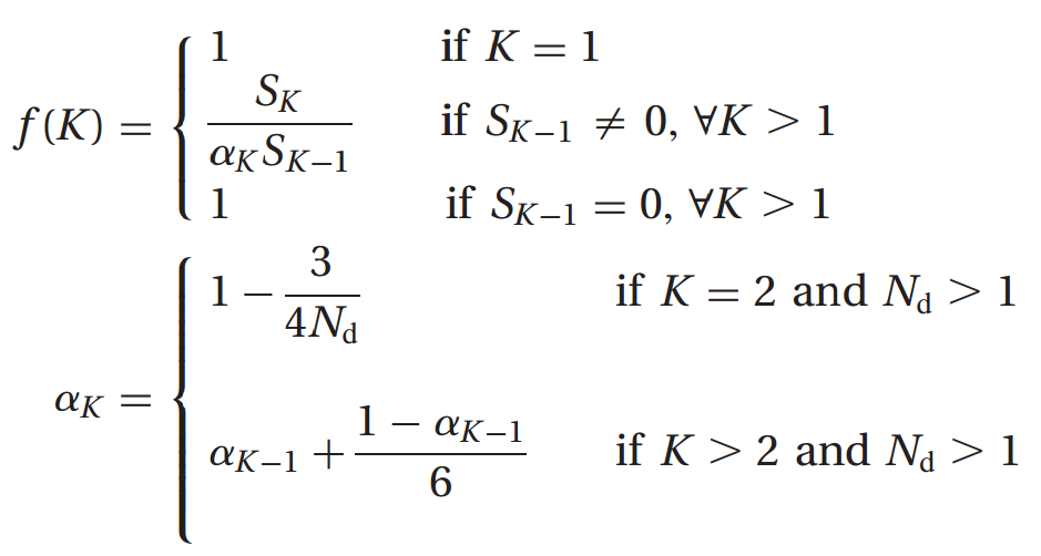
The authors Pham et al. proceed to discuss further constrains that the sought-after function should verify for it to be informative to the problem of selection of K. They finally arrive at the following definition:
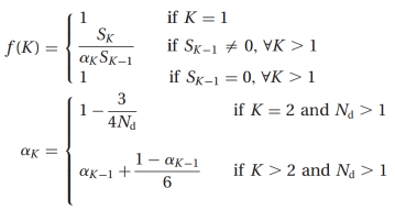
 is the number of dimensions (attributes) of the data set and
  is a weight factor. With this definition, is the ratio of the real distortion to the estimated distortion and decreases when there are areas of concentration in the data distribution. Values of that yield small can be regarded as giving well-defined clusters.
A python implementation of Pham et al. f(K)
Our implementation of the Pham et al. procedure builds on the KMeans and KPlusPlus python classes defined in our article on the k-means++ algorithm. We define a new class that inherits from KPlusPlus and contains a function to compute :
class DetK(KPlusPlus):
    def fK(self, thisk, Skm1=0):
        X = self.X
        Nd = len(X[0])
        a = lambda k, Nd: 1 - 3/(4*Nd) if k == 2 else a(k-1, Nd) + (1-a(k-1, Nd))/6
        self.find_centers(thisk, method='++')
        mu, clusters = self.mu, self.clusters
        Sk = sum([np.linalg.norm(mu[i]-c)**2 \
                 for i in range(thisk) for c in clusters[i]])
        if thisk == 1:
            fs = 1
        elif Skm1 == 0:
            fs = 1
        else:
            fs = Sk/(a(thisk,Nd)*Skm1)
        return fs, Sk
Note the recursive definition of (variable a in the code snapshot above) and the fact that the computation of  for
for  requires knowing the value of
  , which is passed as input parameter to the function.
This article aims at showing that the Pham et al. procedure works and is computationally more efficient than the gap statistic. Therefore, we will code up the algorithm for the gap statistic within the same class DetK, so that we can run both procedures simultaneously. The full code is below the fold:
class DetK(KPlusPlus):
    def fK(self, thisk, Skm1=0):
        X = self.X
        Nd = len(X[0])
        a = lambda k, Nd: 1 - 3/(4*Nd) if k == 2 else a(k-1, Nd) + (1-a(k-1, Nd))/6
        self.find_centers(thisk, method='++')
        mu, clusters = self.mu, self.clusters
        Sk = sum([np.linalg.norm(mu[i]-c)**2 \
                 for i in range(thisk) for c in clusters[i]])
        if thisk == 1:
            fs = 1
        elif Skm1 == 0:
            fs = 1
        else:
            fs = Sk/(a(thisk,Nd)*Skm1)
        return fs, Sk

    def _bounding_box(self):
        X = self.X
        xmin, xmax = min(X,key=lambda a:a[0])[0], max(X,key=lambda a:a[0])[0]
        ymin, ymax = min(X,key=lambda a:a[1])[1], max(X,key=lambda a:a[1])[1]
        return (xmin,xmax), (ymin,ymax)

    def gap(self, thisk):
        X = self.X
        (xmin,xmax), (ymin,ymax) = self._bounding_box()
        self.init_centers(thisk)
        self.find_centers(thisk, method='++')
        mu, clusters = self.mu, self.clusters
        Wk = np.log(sum([np.linalg.norm(mu[i]-c)**2/(2*len(c)) \
                    for i in range(thisk) for c in clusters[i]]))
        # Create B reference datasets
        B = 10
        BWkbs = zeros(B)
        for i in range(B):
            Xb = []
            for n in range(len(X)):
                Xb.append([random.uniform(xmin,xmax), \
                          random.uniform(ymin,ymax)])
            Xb = np.array(Xb)
            kb = DetK(thisk, X=Xb)
            kb.init_centers(thisk)
            kb.find_centers(thisk, method='++')
            ms, cs = kb.mu, kb.clusters
            BWkbs[i] = np.log(sum([np.linalg.norm(ms[j]-c)**2/(2*len(c)) \
                              for j in range(thisk) for c in cs[j]]))
        Wkb = sum(BWkbs)/B
        sk = np.sqrt(sum((BWkbs-Wkb)**2)/float(B))*np.sqrt(1+1/B)
        return Wk, Wkb, sk

    def run(self, maxk, which='both'):
        ks = range(1,maxk)
        fs = zeros(len(ks))
        Wks,Wkbs,sks = zeros(len(ks)+1),zeros(len(ks)+1),zeros(len(ks)+1)
        # Special case K=1
        self.init_centers(1)
        if which == 'f':
            fs[0], Sk = self.fK(1)
        elif which == 'gap':
            Wks[0], Wkbs[0], sks[0] = self.gap(1)
        else:
            fs[0], Sk = self.fK(1)
            Wks[0], Wkbs[0], sks[0] = self.gap(1)
        # Rest of Ks
        for k in ks[1:]:
            self.init_centers(k)
            if which == 'f':
                fs[k-1], Sk = self.fK(k, Skm1=Sk)
            elif which == 'gap':
                Wks[k-1], Wkbs[k-1], sks[k-1] = self.gap(k)
            else:
                fs[k-1], Sk = self.fK(k, Skm1=Sk)
                Wks[k-1], Wkbs[k-1], sks[k-1] = self.gap(k)
        if which == 'f':
            self.fs = fs
        elif which == 'gap':
            G = []
            for i in range(len(ks)):
                G.append((Wkbs-Wks)[i] - ((Wkbs-Wks)[i+1]-sks[i+1]))
            self.G = np.array(G)
        else:
            self.fs = fs
            G = []
            for i in range(len(ks)):
                G.append((Wkbs-Wks)[i] - ((Wkbs-Wks)[i+1]-sks[i+1]))
            self.G = np.array(G)

    def plot_all(self):
        X = self.X
        ks = range(1, len(self.fs)+1)
        fig = plt.figure(figsize=(18,5))
        # Plot 1
        ax1 = fig.add_subplot(131)
        ax1.set_xlim(-1,1)
        ax1.set_ylim(-1,1)
        ax1.plot(zip(*X)[0], zip(*X)[1], '.', alpha=0.5)
        tit1 = 'N=%s' % (str(len(X)))
        ax1.set_title(tit1, fontsize=16)
        # Plot 2
        ax2 = fig.add_subplot(132)
        ax2.set_ylim(0, 1.25)
        ax2.plot(ks, self.fs, 'ro-', alpha=0.6)
        ax2.set_xlabel('Number of clusters K', fontsize=16)
        ax2.set_ylabel('f(K)', fontsize=16)
        foundfK = np.where(self.fs == min(self.fs))[0][0] + 1
        tit2 = 'f(K) finds %s clusters' % (foundfK)
        ax2.set_title(tit2, fontsize=16)
        # Plot 3
        ax3 = fig.add_subplot(133)
        ax3.bar(ks, self.G, alpha=0.5, color='g', align='center')
        ax3.set_xlabel('Number of clusters K', fontsize=16)
        ax3.set_ylabel('Gap', fontsize=16)
        foundG = np.where(self.G > 0)[0][0] + 1
        tit3 = 'Gap statistic finds %s clusters' % (foundG)
        ax3.set_title(tit3, fontsize=16)
        ax3.xaxis.set_ticks(range(1,len(ks)+1))
        plt.savefig('detK_N%s.png' % (str(len(X))), \
                     bbox_inches='tight', dpi=100)
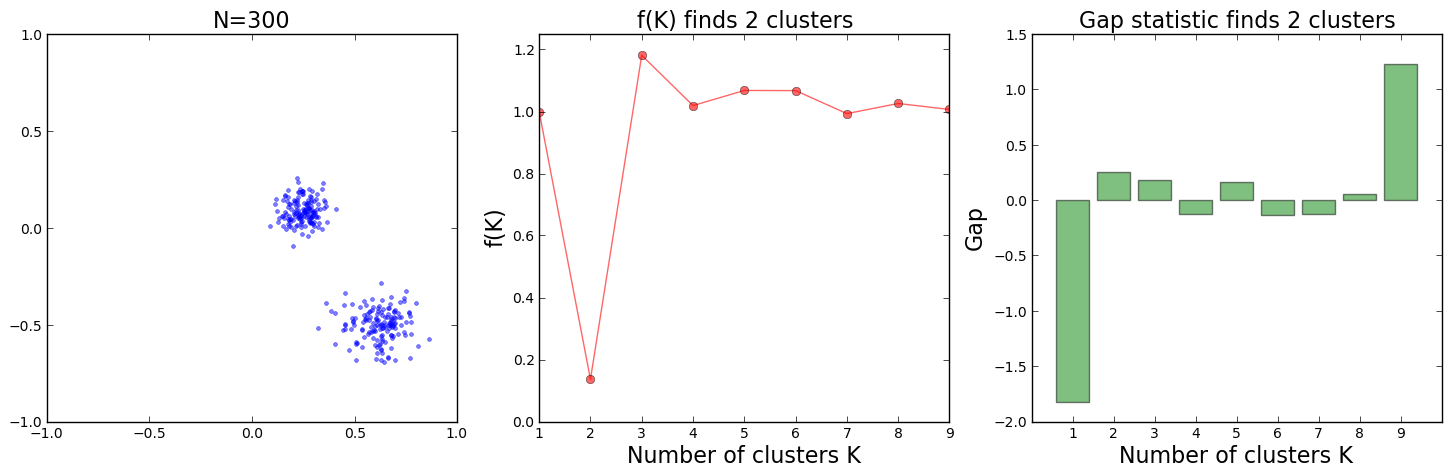
For a first experiment comparing the Pham et al. and the gap statistic approaches, we create a data set comprising 300 points around 2 Gaussian-distributed clusters. We run both methods to select spanning the values  . (The function
 run from class DetK takes a value  as input and checks all values such that
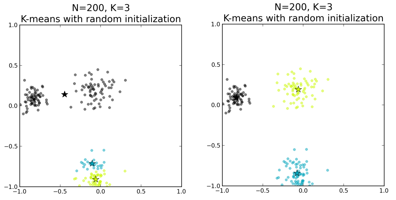
  .) Note that every run of the k-means clustering algorithm for different values of is preceded by the k-means++ initialization algorithm, to prevent landing at suboptimal clustering solutions.
To run a full comparison of both methods, the following simple commands are invoked:
kpp = DetK(2, N=300)
kpp.run(10)
kpp.plot_all()
This produces the following result plots:

According to Pham et al. lower values of , and especially values  are an indication of cluster-like features in the data at that particular . In the case of
  , the global minimum of in the central plot leaves no doubt that this is the right value to choose for this particular data configuration. The gap statistic, depicted in the plot on the right, yields the same result of . Remember that the optimal with the gap statistic is the smallest value for which the gap quantity becomes positive.
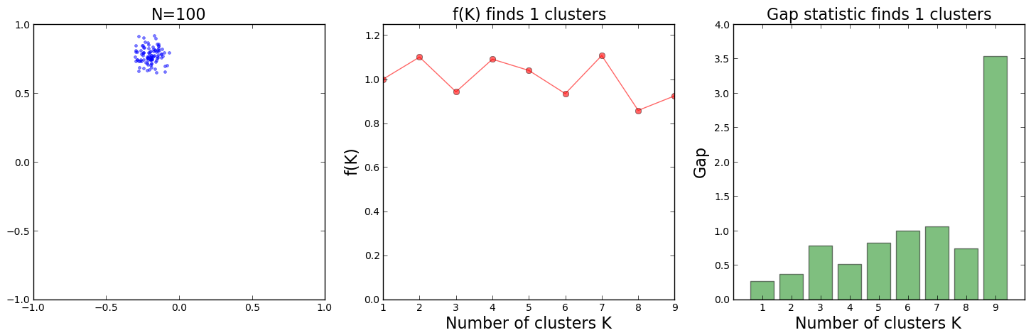
Similarly, we can analyze a data set consisting of 100 points around a single cluster. The results are shown in the plots below. We observe how the function does not show any prominent valley or value for which for any of the surveyed s. According to the Pham et al. paper, this is an indication of no clustering, as is the case. The gap statistic agrees that there is no more than one cluster in this case.

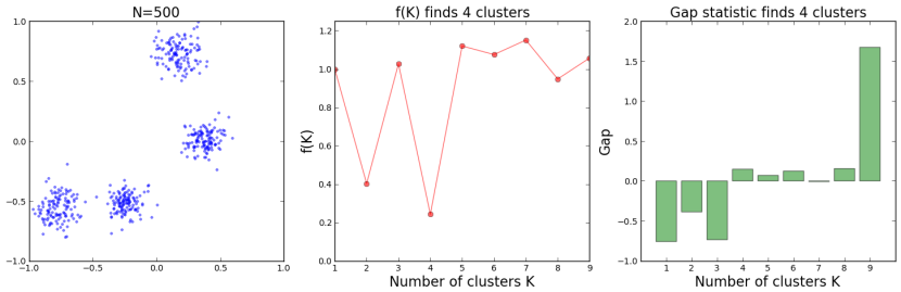
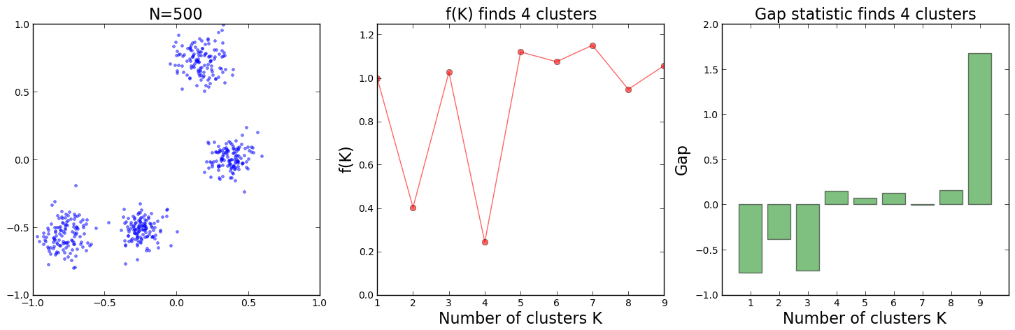
Finally, let us look at two cases, both with 500 data points around 4 clusters. Below are the plots of the results:
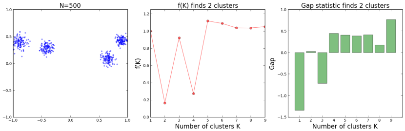
For the data distribution on the top, one can see that the 4 clusters are positioned in such a way that they could also be interpreted as 2 clusters made of 2 subclusters each. The detects this configuration and suggests 2 possible values of , with a slight preference for over  . The gap statistic changes sign at , albeit barely, and it does it again and more clearly at . In both cases, a strict application of the rules prescribed to select the correct does lead to a rather suboptimal, or at least dubious, choice.
In the bottom plot however, the 4 clusters are somehow more evenly spreaded and both algorithms succeed at identifying . The method still shows a relative minimum at , indicating a potentially alternative clustering.
Performance comparison of f(K) and the gap statistic
If both methods to select the optimal for k-means clustering yield similar results, one should ask about the relative performance of them in real-life data science clustering problems. It is straightforward to predict that the gap statistic, with its need for running the k-means algorithm multiple times to create a Monte Carlo reference distribution, will necessarily be a poorer performer. We can easily test this hypothesis with our code by running both approaches and timing them using the IPython magic %time function. For a data set with  :
:
%time kpp.run(10, which='f')
CPU times: user 2.72 s, sys: 0.00 s, total: 2.72 s

Wall time: 2.90 s
%time kpp.run(10, which='gap')
CPU times: user 51.30 s, sys: 0.01 s, total: 51.31 s

Wall time: 51.40 s
In this particular example, the method is more than one order of magnitude more performant than the gap statistic, and this comparison looks worse for the latter the more data we take into consideration and the larger the number  employed for generating the reference distributions.
Table-top data experiment take-away message
The estimation of the optimal number of clusters within a set of data points is a very important problem, as most clustering algorithms need that parameter as input in order to group the data. Many methods have been proposed to find the proper , among which the approach proposed by Pham et al. in 2004 seems to offer a very straightforward and performant solution. The estimation of the function over the desired range of test values for offers an immediate way of assessing when the cluster-like features appear and allows to choose among a best value and other alternatives. A comparison in performance with the gap statistic method of Tibshirani et al. concludes that the is computationally advantageous.


 ,
, uniformly at random from X. Compute the vector containing the square distances between all points in the dataset and
 from X randomly drawn from the probability distribution

 and recompute the distance vector as
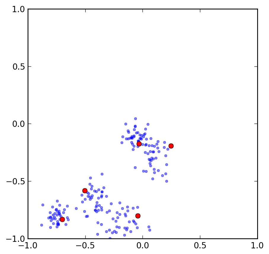
![r \in [0,1]](https://s0.wp.com/latex.php?latex=r+%5Cin+%5B0%2C1%5D&bg=ffffff&fg=000000&s=1&c=20201002) and finding the point corresponding to the segment of the partition where that
and finding the point corresponding to the segment of the partition where that  value falls, we are effectively choosing a point drawn according to the desired probability distribution. On the right is a plot showing the results of the algorithm for 200 points and 5 clusters.
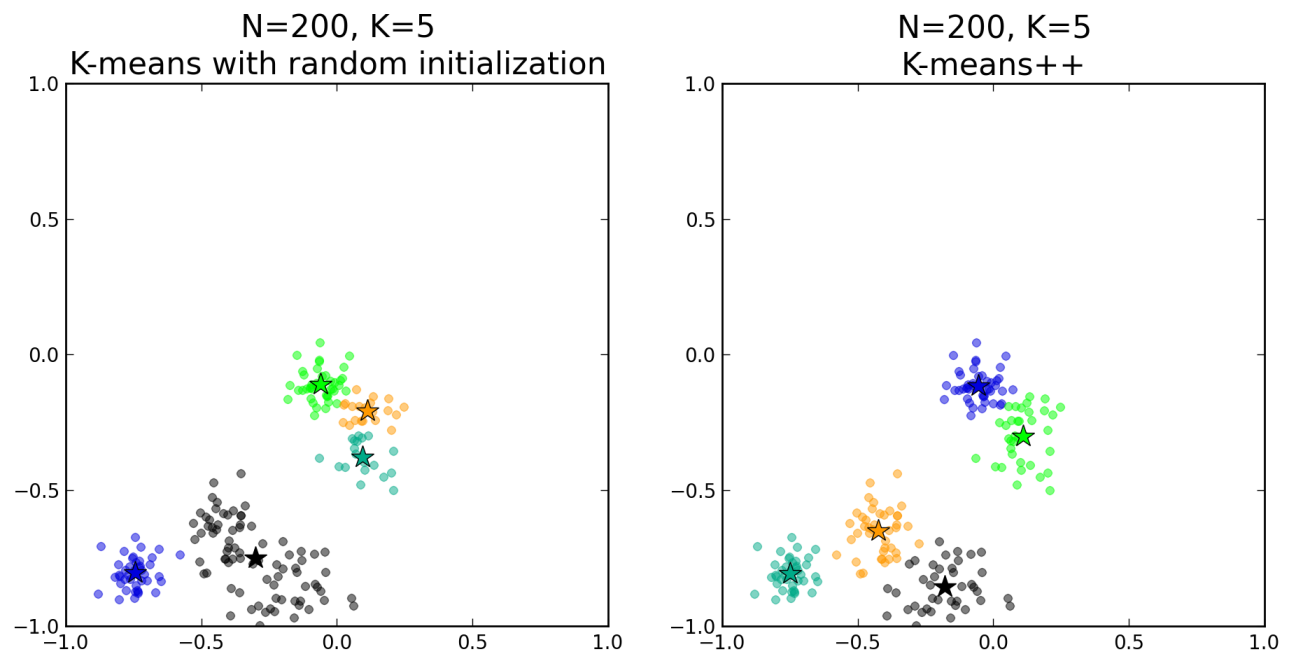
