Finding the K in K-Means Clustering

December 27, 2013

A couple of weeks ago, here at The Data Science Lab we showed how Lloyd’s algorithm can be used to cluster points using k-means with a simple python implementation. We also produced interesting visualizations of the Voronoi tessellation induced by the clustering. At the end of the post we hinted at some of the shortcomings of this clustering procedure. The basic k-means is an extremely simple and efficient algorithm. However, it assumes prior knowledge of the data in order to choose the appropriate K. Other disadvantages are the sensitivity of the final clusters to the selection of the initial centroids and the fact that the algorithm can produce empty clusters. In today’s post, and by popular request, we are going to have a look at the first question, namely how to find the appropriate K to use in the k-means clustering procedure.

Meaning and purpose of clustering, and the elbow method

Clustering consist of grouping objects in sets, such that objects within a cluster are as similar as possible, whereas objects from different clusters are as dissimilar as possible. Thus, the optimal clustering is somehow subjective and dependent on the characteristic used for determining similarities, as well as on the level of detail required from the partitions. For the purpose of our clustering experiment we use clusters derived from Gaussian distributions, i.e. globular in nature, and look only at the usual definition of Euclidean distance between points in a two-dimensional space to determine intra- and inter-cluster similarity.

The following measure represents the sum of intra-cluster distances between points in a given cluster containing points:

.

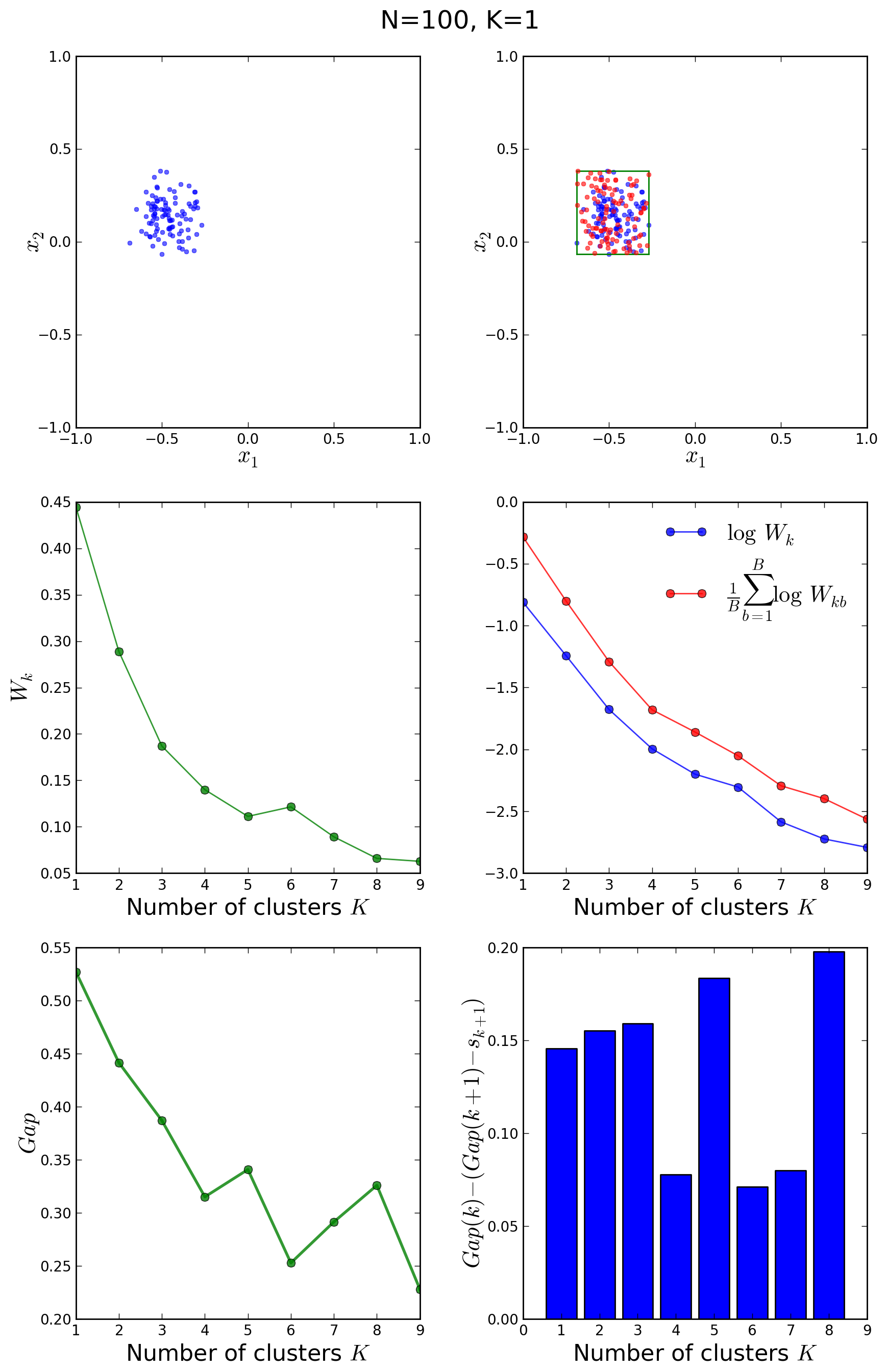
Adding the normalized intra-cluster sums of squares gives a measure of the compactness of our clustering:

.

This variance quantity is the basis of a naive procedure to determine the optimal number of clusters: the elbow method.

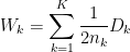
If you graph the percentage of variance explained by the clusters against the number of clusters, the first clusters will add much information (explain a lot of variance), but at some point the marginal gain will drop, giving an angle in the graph. The number of clusters are chosen at this point, hence the “elbow criterion”.

But as Wikipedia promptly explains, this “elbow” cannot always be unambiguously identified. In this post we will show a more sophisticated method that provides a statistical procedure to formalize the “elbow” heuristic.

The gap statistic

The gap statistic was developed by Stanford researchers Tibshirani, Walther and Hastie in their 2001 paper. The idea behind their approach was to find a way to standardize the comparison of with a null reference distribution of the data, i.e. a distribution with no obvious clustering. Their estimate for the optimal number of clusters is the value for which falls the farthest below this reference curve. This information is contained in the following formula for the gap statistic:

.

The reference datasets are in our case generated by sampling uniformly from the original dataset’s bounding box (see green box in the upper right plot of the figures below). To obtain the estimate we compute the average of copies for , each of which is generated with a Monte Carlo sample from the reference distribution. Those from the Monte Carlo replicates exhibit a standard deviation which, accounting for the simulation error, is turned into the quantity

.

Finally, the optimal number of clusters is the smallest such that .

A Python implementation of the algorithm

The computation of the gap statistic involves the following steps (see original paper):

• Cluster the observed data, varying the number of clusters from , and compute the corresponding .
• Generate reference data sets and cluster each of them with varying number of clusters . Compute the estimated gap statistic .
• With , compute the standard deviation and define .
• Choose the number of clusters as the smallest such that .

Our python implementation makes use of the find_centers(X, K) function defined in this post. The quantity is computed as follows:

def Wk(mu, clusters):
    K = len(mu)
    return sum([np.linalg.norm(mu[i]-c)**2/(2*len(c)) \
               for i in range(K) for c in clusters[i]])

The gap statistic is implemented in the following code snapshot. Note that we use for the reference datasets and we span values of from 1 to 9.

def bounding_box(X):
    xmin, xmax = min(X,key=lambda a:a[0])[0], max(X,key=lambda a:a[0])[0]
    ymin, ymax = min(X,key=lambda a:a[1])[1], max(X,key=lambda a:a[1])[1]
    return (xmin,xmax), (ymin,ymax)

def gap_statistic(X):
    (xmin,xmax), (ymin,ymax) = bounding_box(X)
    # Dispersion for real distribution
    ks = range(1,10)
    Wks = zeros(len(ks))
    Wkbs = zeros(len(ks))
    sk = zeros(len(ks))
    for indk, k in enumerate(ks):
        mu, clusters = find_centers(X,k)
        Wks[indk] = np.log(Wk(mu, clusters))
        # Create B reference datasets
        B = 10
        BWkbs = zeros(B)
        for i in range(B):
            Xb = []
            for n in range(len(X)):
                Xb.append([random.uniform(xmin,xmax),
                          random.uniform(ymin,ymax)])
            Xb = np.array(Xb)
            mu, clusters = find_centers(Xb,k)
            BWkbs[i] = np.log(Wk(mu, clusters))
        Wkbs[indk] = sum(BWkbs)/B
        sk[indk] = np.sqrt(sum((BWkbs-Wkbs[indk])**2)/B)
    sk = sk*np.sqrt(1+1/B)
    return(ks, Wks, Wkbs, sk)

Finding the K

We shall now apply our algorithm to diverse distributions and see how it performs. Using the init_board_gauss(N, k) function defined in our previous post, we produce an ensemble of 200 data points normally distributed around 3 centers and run the gap statistic on them.

X = init_board_gauss(200,3)
ks, logWks, logWkbs, sk = gap_statistic(X)

The following plot gives an idea of what is happening:

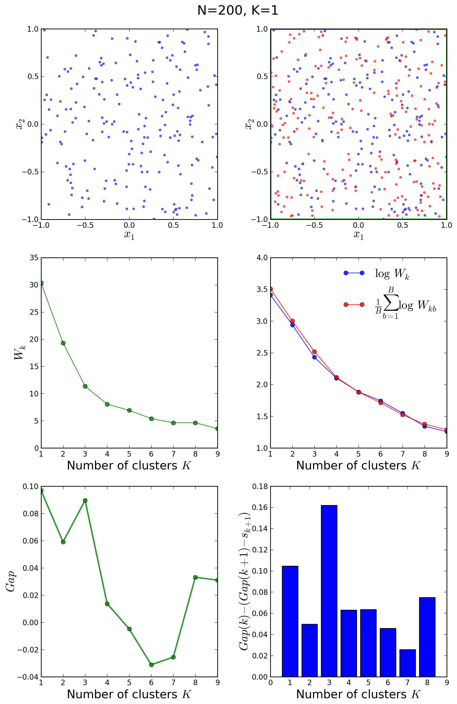
The upper left plot shows the target distribution with 3 clusters. On the right is its bounding box and one Monte Carlo sample drawn from a uniform reference distribution within that rectangle. In the middle left we see the plot of that is used to determine with the elbow method. Indeed a knee-like feature is observed at , however the gap statistic is a better way of formalizing this phenomenon. On the right is the comparison of for the original and averaged reference distributions. Finally, the bottom plots show the gap quantity on the left, with a clear peak at the correct and the criteria for choosing it on the right. The correct is the smallest for which the quantity plotted in blue bars becomes positive. The optimal number is correctly guessed by the algorithm as .

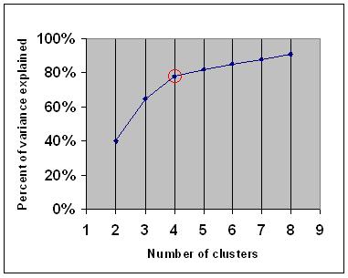
Let us now have a look at another example with 400 points around 5 clusters:

In this case, the elbow method would not have been conclusive, however the gap statistic correctly shows a peak in the gap at and the bar plot changes sign at the same correct value.

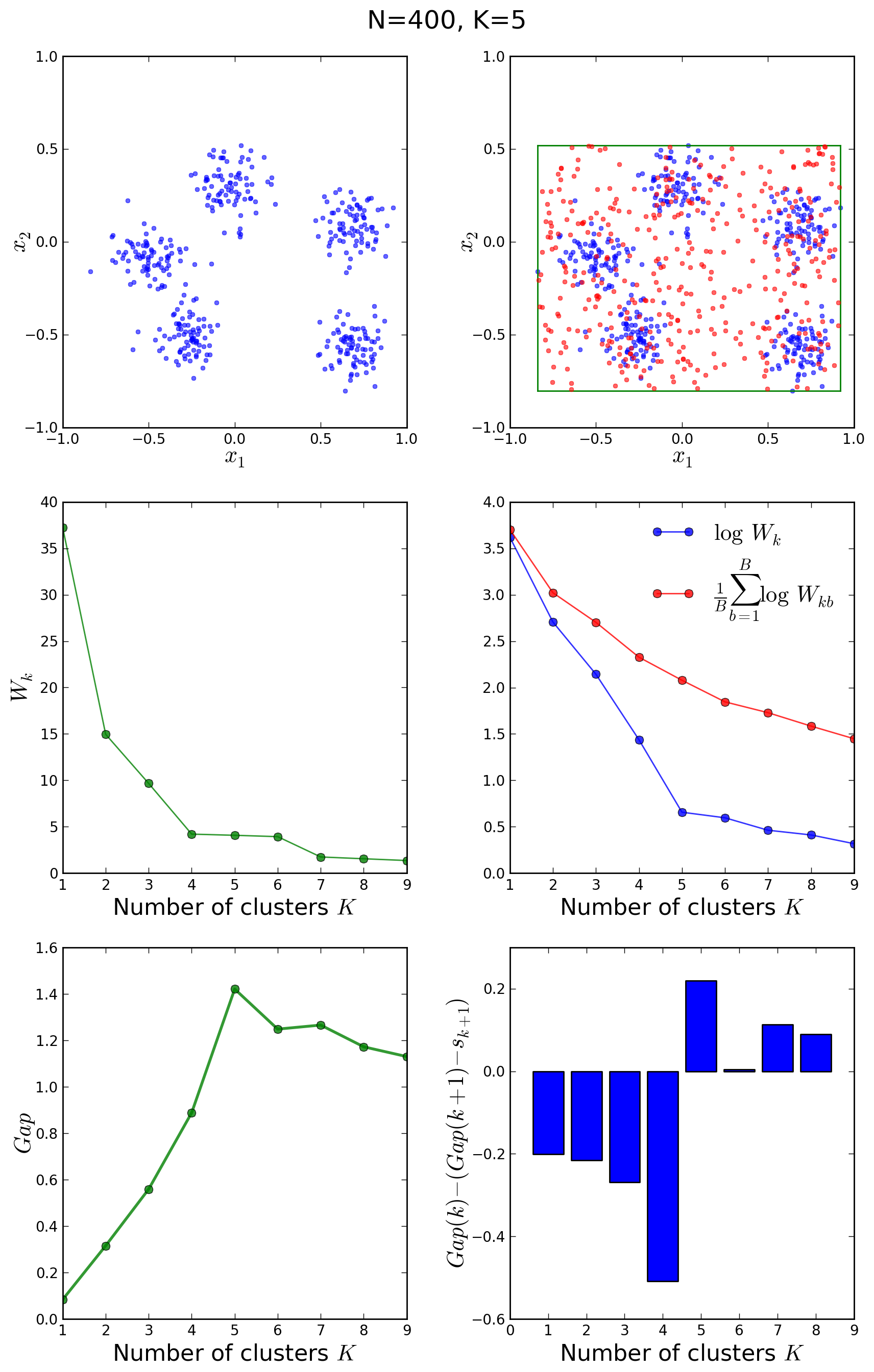
Similarly, we can study what happens when the data points are clustered around a single centroid:

It is clear in the above figures that the original and the reference distributions in the middle right plot follow the same decay law, so that no abrupt fall-off of the blue curve with respect to the red one is observed at any . The bar plot shows positive values for the entire range. We conclude that is the correct clustering.

Finally, let us have a look at a uniform, non-clustered distribution of 200 points, generated with the init_board(N) function defined in our previous post:

In this case, the algorithm also guesses correctly, and it is clear from the middle right plot that both the original and the reference distributions follow exactly the same decay law, since they are essentially different samples from the same uniform distribution on [-1,1] x [-1,1]. The gap curve on the bottom left oscillates between local maxima and minima, indicating certain structures within the original distribution originated by statistical fluctuations.

Table-top data experiment take-away message

The estimation of the optimal number of clusters within a set of data points is a very important problem, as most clustering algorithms need that parameter as input in order to group the data. Many methods have been proposed to find the proper , among which the “elbow” method offers a very clear and naive solution based on intra-cluster variance. The gap statistic, proposed by Tobshirani et al. formalizes this approach and offers an easy-to-implement algorithm that successfully finds the correct in the case of globular, Gaussian-distributed, mildly disjoint data distributions.

Update: For a proper initialization of the centroids at the start of the k-means algorithm, we implement the improved k-means++ seeding procedure.

Update: For a comparison of this approach with an alternative method for finding the K in k-means clustering, read this article.

Written by datasciencelab Posted in Experiments Tagged with clustering, gap statistic, k-means, python