Tagged: k-means

January 21, 2014

Selection of K in K-means Clustering, Reloaded

This article follows up on the series devoted to k-means clustering at The Data Science Lab. Previous posts have dealt with how to implement Lloyd’s algorithm for clustering in python, described an improved initialization algorithm for proper seeding of the initial clusters, k-means++, and introduced the gap statistic as a method of finding the optimal K for k-means clustering.

Although the gap statistic, based on a paper by Tibshirani et al was shown to find optimal values for the number of clusters in a variety of cases when the clusters where globular and mildly disjointed, its performance might be hampered by the need of perfoming Monte Carlo simulations to estimate the reference datasets. A reader of this blog, Jonathan Stray, pointed out a potentially superior method for selecting the K in k-means clustering, so let us implement it and compare.

An alternative approach to finding the optimal K

The approach suggested by our reader is based on a publication by Pham, Dimov and Nguyen from 2004. The article is very much worth reading, as it includes an explanation of the drawbacks of the standard k-means algorithm as well as a comprehensive survey on different methods that have been proposed for selecting an optimal number of clusters.

In section 3 of the paper, the authors justify the introduction of a function $f(K)$ to evaluate the quality of the resulting clustering and help decide on the optimal value of $K$ for each data set. Quoting from the paper:

A data set with $n$ objects could be grouped into any number of clusters between 1 and $n$ , which would correspond to the lowest and the highest levels of detail respectively. By specifying different $K$ values, it is possible to assess the results of grouping objects into various numbers of clusters. From this evaluation, more than one $K$ value could be recommended to users, but the ﬁnal selection is made by them.

The goal of a clustering algorithm is to identify regions in which the data points are concentrated. It is also important to analyze the internal distribution of each cluster as well as its relation to other clusters in the data set. The distorsion of a cluster is a measure of the distance between points in a cluster and its centroid:

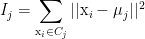
$\displaystyle I_j = \sum_{\mathrm{x}_i \in C_j} ||\mathrm{x}_i - \mu_j ||^2$ .

The global impact of all clusters’ distortions is given by the quantity

$\displaystyle S_k = \sum_{j=1}^K I_j$ .

The authors Pham et al. proceed to discuss further constrains that the sought-after function $f(K)$ should verify for it to be informative to the problem of selection of K. They finally arrive at the following definition:

$N_d$ is the number of dimensions (attributes) of the data set and $\alpha_K$ is a weight factor. With this definition, $f(K)$ is the ratio of the real distortion to the estimated distortion and decreases when there are areas of concentration in the data distribution. Values of $K$ that yield small $f(K)$ can be regarded as giving well-deﬁned clusters.

A python implementation of Pham et al. f(K)

Our implementation of the Pham et al. procedure builds on the KMeans and KPlusPlus python classes defined in our article on the k-means++ algorithm. We define a new class that inherits from KPlusPlus and contains a function to compute $f(K)$ :

class DetK(KPlusPlus):
    def fK(self, thisk, Skm1=0):
        X = self.X
        Nd = len(X[0])
        a = lambda k, Nd: 1 - 3/(4*Nd) if k == 2 else a(k-1, Nd) + (1-a(k-1, Nd))/6
        self.find_centers(thisk, method='++')
        mu, clusters = self.mu, self.clusters
        Sk = sum([np.linalg.norm(mu[i]-c)**2 \
                 for i in range(thisk) for c in clusters[i]])
        if thisk == 1:
            fs = 1
        elif Skm1 == 0:
            fs = 1
        else:
            fs = Sk/(a(thisk,Nd)*Skm1)
        return fs, Sk

Note the recursive definition of $\alpha_K$ (variable a in the code snapshot above) and the fact that the computation of $S_K$ for $K > 1$ requires knowing the value of $S_{K-1}$ , which is passed as input parameter to the function.

This article aims at showing that the Pham et al. procedure works and is computationally more efficient than the gap statistic. Therefore, we will code up the algorithm for the gap statistic within the same class DetK, so that we can run both procedures simultaneously. The full code is below the fold:

class DetK(KPlusPlus):
    def fK(self, thisk, Skm1=0):
        X = self.X
        Nd = len(X[0])
        a = lambda k, Nd: 1 - 3/(4*Nd) if k == 2 else a(k-1, Nd) + (1-a(k-1, Nd))/6
        self.find_centers(thisk, method='++')
        mu, clusters = self.mu, self.clusters
        Sk = sum([np.linalg.norm(mu[i]-c)**2 \
                 for i in range(thisk) for c in clusters[i]])
        if thisk == 1:
            fs = 1
        elif Skm1 == 0:
            fs = 1
        else:
            fs = Sk/(a(thisk,Nd)*Skm1)
        return fs, Sk  

    def _bounding_box(self):
        X = self.X
        xmin, xmax = min(X,key=lambda a:a[0])[0], max(X,key=lambda a:a[0])[0]
        ymin, ymax = min(X,key=lambda a:a[1])[1], max(X,key=lambda a:a[1])[1]
        return (xmin,xmax), (ymin,ymax)        
        
    def gap(self, thisk):
        X = self.X
        (xmin,xmax), (ymin,ymax) = self._bounding_box()
        self.init_centers(thisk)
        self.find_centers(thisk, method='++')
        mu, clusters = self.mu, self.clusters
        Wk = np.log(sum([np.linalg.norm(mu[i]-c)**2/(2*len(c)) \
                    for i in range(thisk) for c in clusters[i]]))
        # Create B reference datasets
        B = 10
        BWkbs = zeros(B)
        for i in range(B):
            Xb = []
            for n in range(len(X)):
                Xb.append([random.uniform(xmin,xmax), \
                          random.uniform(ymin,ymax)])
            Xb = np.array(Xb)
            kb = DetK(thisk, X=Xb)
            kb.init_centers(thisk)
            kb.find_centers(thisk, method='++')
            ms, cs = kb.mu, kb.clusters
            BWkbs[i] = np.log(sum([np.linalg.norm(ms[j]-c)**2/(2*len(c)) \
                              for j in range(thisk) for c in cs[j]]))
        Wkb = sum(BWkbs)/B
        sk = np.sqrt(sum((BWkbs-Wkb)**2)/float(B))*np.sqrt(1+1/B)
        return Wk, Wkb, sk
    
    def run(self, maxk, which='both'):
        ks = range(1,maxk)
        fs = zeros(len(ks))
        Wks,Wkbs,sks = zeros(len(ks)+1),zeros(len(ks)+1),zeros(len(ks)+1)
        # Special case K=1
        self.init_centers(1)
        if which == 'f':
            fs[0], Sk = self.fK(1)
        elif which == 'gap':
            Wks[0], Wkbs[0], sks[0] = self.gap(1)
        else:
            fs[0], Sk = self.fK(1)
            Wks[0], Wkbs[0], sks[0] = self.gap(1)
        # Rest of Ks
        for k in ks[1:]:
            self.init_centers(k)
            if which == 'f':
                fs[k-1], Sk = self.fK(k, Skm1=Sk)
            elif which == 'gap':
                Wks[k-1], Wkbs[k-1], sks[k-1] = self.gap(k)
            else:
                fs[k-1], Sk = self.fK(k, Skm1=Sk)
                Wks[k-1], Wkbs[k-1], sks[k-1] = self.gap(k)
        if which == 'f':
            self.fs = fs
        elif which == 'gap':
            G = []
            for i in range(len(ks)):
                G.append((Wkbs-Wks)[i] - ((Wkbs-Wks)[i+1]-sks[i+1]))
            self.G = np.array(G)
        else:
            self.fs = fs
            G = []
            for i in range(len(ks)):
                G.append((Wkbs-Wks)[i] - ((Wkbs-Wks)[i+1]-sks[i+1]))
            self.G = np.array(G)
    
    def plot_all(self):
        X = self.X
        ks = range(1, len(self.fs)+1)
        fig = plt.figure(figsize=(18,5))
        # Plot 1
        ax1 = fig.add_subplot(131)
        ax1.set_xlim(-1,1)
        ax1.set_ylim(-1,1)
        ax1.plot(zip(*X)[0], zip(*X)[1], '.', alpha=0.5)
        tit1 = 'N=%s' % (str(len(X)))
        ax1.set_title(tit1, fontsize=16)
        # Plot 2
        ax2 = fig.add_subplot(132)
        ax2.set_ylim(0, 1.25)
        ax2.plot(ks, self.fs, 'ro-', alpha=0.6)
        ax2.set_xlabel('Number of clusters K', fontsize=16)
        ax2.set_ylabel('f(K)', fontsize=16) 
        foundfK = np.where(self.fs == min(self.fs))[0][0] + 1
        tit2 = 'f(K) finds %s clusters' % (foundfK)
        ax2.set_title(tit2, fontsize=16)
        # Plot 3
        ax3 = fig.add_subplot(133)
        ax3.bar(ks, self.G, alpha=0.5, color='g', align='center')
        ax3.set_xlabel('Number of clusters K', fontsize=16)
        ax3.set_ylabel('Gap', fontsize=16)
        foundG = np.where(self.G > 0)[0][0] + 1
        tit3 = 'Gap statistic finds %s clusters' % (foundG)
        ax3.set_title(tit3, fontsize=16)
        ax3.xaxis.set_ticks(range(1,len(ks)+1))
        plt.savefig('detK_N%s.png' % (str(len(X))), \
                     bbox_inches='tight', dpi=100)

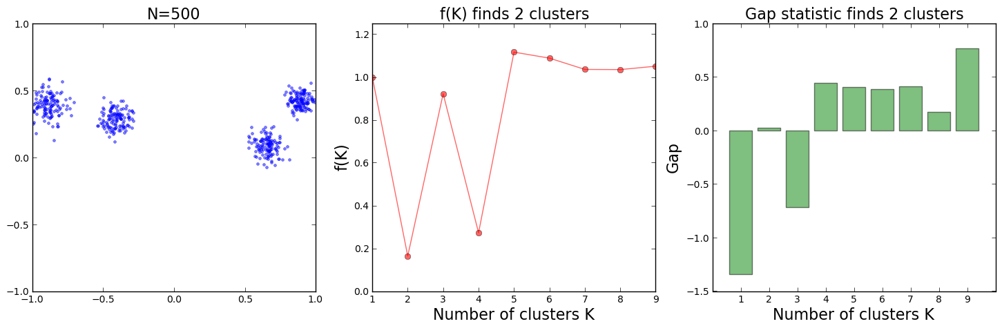
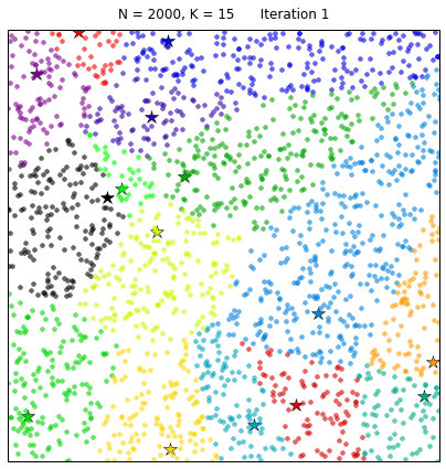
For a first experiment comparing the Pham et al. and the gap statistic approaches, we create a data set comprising 300 points around 2 Gaussian-distributed clusters. We run both methods to select $K$ spanning the values $K=1, \ldots, 9$ . (The function run from class DetK takes a value $k_{thr}$ as input and checks all values such that $k < k_{thr}$ .) Note that every run of the k-means clustering algorithm for different values of $K$ is preceded by the k-means++ initialization algorithm, to prevent landing at suboptimal clustering solutions.

To run a full comparison of both methods, the following simple commands are invoked:

kpp = DetK(2, N=300)
kpp.run(10)
kpp.plot_all()

This produces the following result plots:

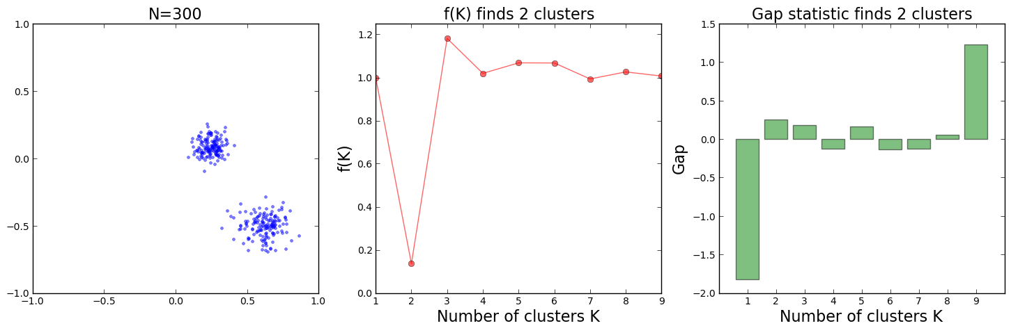
According to Pham et al. lower values of $f(K)$ , and especially values $f(K) < 0.85$ are an indication of cluster-like features in the data at that particular $K$ . In the case of $K=2$ , the global minimum of $f(K)$ in the central plot leaves no doubt that this is the right value to choose for this particular data configuration. The gap statistic, depicted in the plot on the right, yields the same result of $K=2$ . Remember that the optimal $K$ with the gap statistic is the smallest value for which the gap quantity becomes positive.

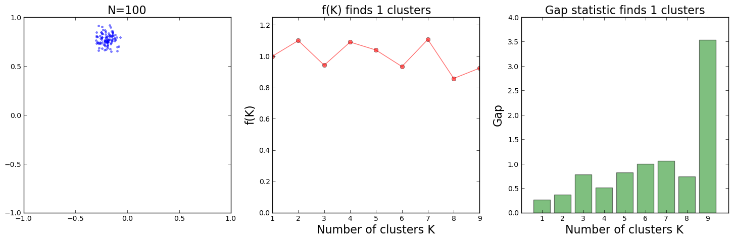
Similarly, we can analyze a data set consisting of 100 points around a single cluster. The results are shown in the plots below. We observe how the function $f(K)$ does not show any prominent valley or value for which $f(K) < 0.85$ for any of the surveyed $K$ s. According to the Pham et al. paper, this is an indication of no clustering, as is the case. The gap statistic agrees that there is no more than one cluster in this case.

Finally, let us look at two cases, both with 500 data points around 4 clusters. Below are the plots of the results:

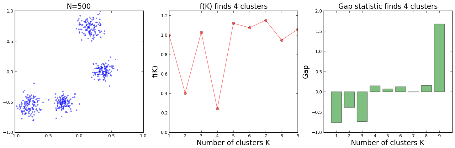
For the data distribution on the top, one can see that the 4 clusters are positioned in such a way that they could also be interpreted as 2 clusters made of 2 subclusters each. The $f(K)$ detects this configuration and suggests 2 possible values of $K$ , with a slight preference for $K=2$ over $K=4$ . The gap statistic changes sign at $K=2$ , albeit barely, and it does it again and more clearly at $K=4$ . In both cases, a strict application of the rules prescribed to select the correct $K$ does lead to a rather suboptimal, or at least dubious, choice.

In the bottom plot however, the 4 clusters are somehow more evenly spreaded and both algorithms succeed at identifying $K=4$ . The $f(K)$ method still shows a relative minimum at $K=2$ , indicating a potentially alternative clustering.

Performance comparison of f(K) and the gap statistic

If both methods to select the optimal $K$ for k-means clustering yield similar results, one should ask about the relative performance of them in real-life data science clustering problems. It is straightforward to predict that the gap statistic, with its need for running the k-means algorithm multiple times to create a Monte Carlo reference distribution, will necessarily be a poorer performer. We can easily test this hypothesis with our code by running both approaches and timing them using the IPython magic %time function. For a data set with $N = 500$ :

%time kpp.run(10, which='f')

CPU times: user 2.72 s, sys: 0.00 s, total: 2.72 s Wall time: 2.90 s

%time kpp.run(10, which='gap')

CPU times: user 51.30 s, sys: 0.01 s, total: 51.31 s Wall time: 51.40 s

In this particular example, the $f(K)$ method is more than one order of magnitude more performant than the gap statistic, and this comparison looks worse for the latter the more data we take into consideration and the larger the number $B$ employed for generating the reference distributions.

Table-top data experiment take-away message

The estimation of the optimal number of clusters within a set of data points is a very important problem, as most clustering algorithms need that parameter as input in order to group the data. Many methods have been proposed to find the proper $K$ , among which the approach proposed by Pham et al. in 2004 seems to offer a very straightforward and performant solution. The estimation of the function $f(K)$ over the desired range of test values for $K$ offers an immediate way of assessing when the cluster-like features appear and allows to choose among a best value and other alternatives. A comparison in performance with the gap statistic method of Tibshirani et al. concludes that the $f(K)$ is computationally advantageous.

January 15, 2014

Improved Seeding For Clustering With K-Means++

Clustering data into subsets is an important task for many data science applications. At The Data Science Lab we have illustrated how Lloyd’s algorithm for k-means clustering works, including snapshots of python code to visualize the iterative clustering steps. One of the issues with the procedure is that

this algorithm does not supply information as to which K for the k-means is optimal; that has to be found out by alternative methods,

so that we went a step further and coded up the gap statistic to find the proper k for k-means clustering. In combination with the clustering algorithm, the gap statistic allows to estimate the best value for k among those in a given range.

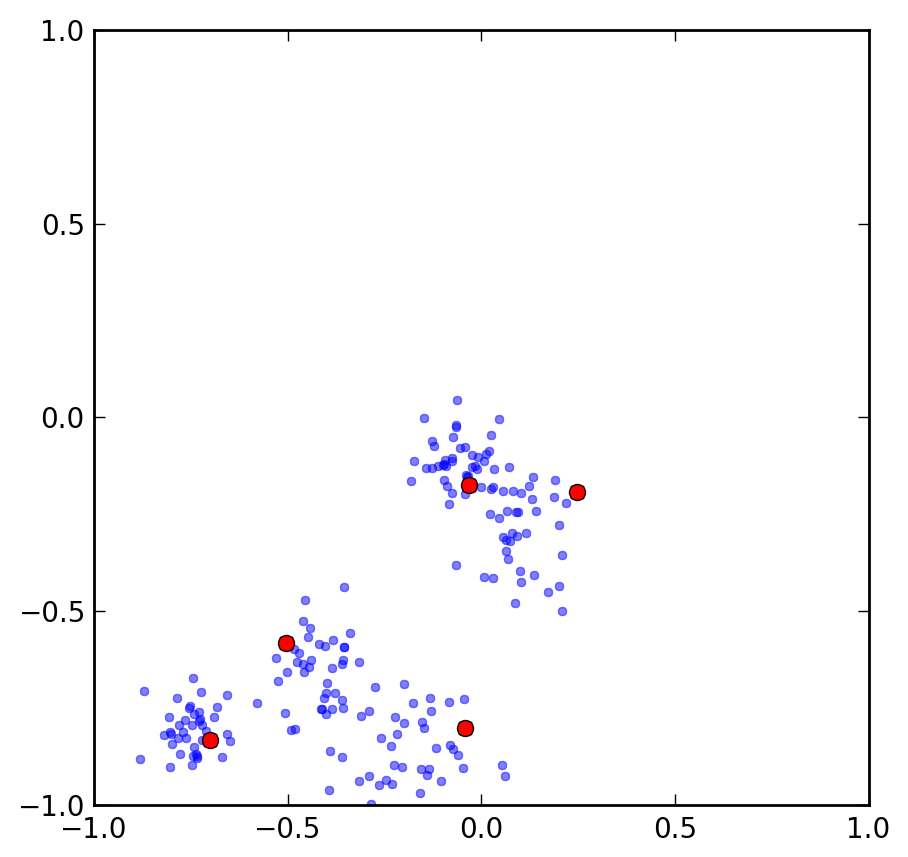
An additional problem with the standard k-means procedure still remains though, as shown by the image on the right, where a poor random initialization of the centroids leads to suboptimal clustering:

If the target distribution is disjointedly clustered and only one instantiation of Lloyd’s algorithm is used, the danger exists that the local minimum reached is not the optimal solution.

The initialization problem for the k-means algorithm is an important practical one, and has been discussed extensively. It is desirable to augment the standard k-means clustering procedure with a robust initialization mechanism that guarantees convergence to the optimal solution.

k-means++: the advantages of careful seeding

A solution called k-means++ was proposed in 2007 by Arthur and Vassilvitskii. This algorithm comes with a theoretical guarantee to find a solution that is O(log k) competitive to the optimal k-means solution. It is also fairly simple to describe and implement. Starting with a dataset X of N points $(\mathrm{x}_1, \ldots, \mathrm{x}_N)$ ,

choose an initial center $c_1$ uniformly at random from X. Compute the vector containing the square distances between all points in the dataset and $c_1$ : $D_i^2 = ||\mathrm{x}_i - c_1 ||^2$
choose a second center $c_2$ from X randomly drawn from the probability distribution $D_i^2 / \sum_j D_j^2$
recompute the distance vector as $D_i^2 = \mathrm{min} \left(||\mathrm{x}_i - c_1 ||^2, ||\mathrm{x}_i - c_2 ||^2\right)$
choose a successive center $c_l$ and recompute the distance vector as $D_i^2 = \mathrm{min} \left(||\mathrm{x}_i - c_1 ||^2, \ldots, ||\mathrm{x}_i - c_l ||^2\right)$
when exactly k centers have been chosen, finalize the initialization phase and proceed with the standard k-means algorithm

The interested reader can find a review of the k-means++ algorithm at normaldeviate, a survey of implementations in several languages at rosettacode and a ready-to-use solution in pandas by Jack Maney in github.

A python implementation of the k-means++ algorithm

Out python implementation of the k-means++ algorithm builds on the code for standard k-means shown in the previous post. The KMeans class defined below contains all necessary functions and methods to generate toy data and run the Lloyd’s clustering algorithm on it:

class KMeans():
    def __init__(self, K, X=None, N=0):
        self.K = K
        if X == None:
            if N == 0:
                raise Exception("If no data is provided, \
                                 a parameter N (number of points) is needed")
            else:
                self.N = N
                self.X = self._init_board_gauss(N, K)
        else:
            self.X = X
            self.N = len(X)
        self.mu = None
        self.clusters = None
        self.method = None

    def _init_board_gauss(self, N, k):
        n = float(N)/k
        X = []
        for i in range(k):
            c = (random.uniform(-1,1), random.uniform(-1,1))
            s = random.uniform(0.05,0.15)
            x = []
            while len(x) < n:
                a,b = np.array([np.random.normal(c[0],s),np.random.normal(c[1],s)])
                # Continue drawing points from the distribution in the range [-1,1]
                if abs(a) and abs(b)<1:
                    x.append([a,b])
            X.extend(x)
        X = np.array(X)[:N]
        return X

    def plot_board(self):
        X = self.X
        fig = plt.figure(figsize=(5,5))
        plt.xlim(-1,1)
        plt.ylim(-1,1)
        if self.mu and self.clusters:
            mu = self.mu
            clus = self.clusters
            K = self.K
            for m, clu in clus.items():
                cs = cm.spectral(1.*m/self.K)
                plt.plot(mu[m][0], mu[m][1], 'o', marker='*', \
                         markersize=12, color=cs)
                plt.plot(zip(*clus[m])[0], zip(*clus[m])[1], '.', \
                         markersize=8, color=cs, alpha=0.5)
        else:
            plt.plot(zip(*X)[0], zip(*X)[1], '.', alpha=0.5)
        if self.method == '++':
            tit = 'K-means++'
        else:
            tit = 'K-means with random initialization'
        pars = 'N=%s, K=%s' % (str(self.N), str(self.K))
        plt.title('\n'.join([pars, tit]), fontsize=16)
        plt.savefig('kpp_N%s_K%s.png' % (str(self.N), str(self.K)), \
                    bbox_inches='tight', dpi=200)

    def _cluster_points(self):
        mu = self.mu
        clusters  = {}
        for x in self.X:
            bestmukey = min([(i[0], np.linalg.norm(x-mu[i[0]])) \
                             for i in enumerate(mu)], key=lambda t:t[1])[0]
            try:
                clusters[bestmukey].append(x)
            except KeyError:
                clusters[bestmukey] = [x]
        self.clusters = clusters

    def _reevaluate_centers(self):
        clusters = self.clusters
        newmu = []
        keys = sorted(self.clusters.keys())
        for k in keys:
            newmu.append(np.mean(clusters[k], axis = 0))
        self.mu = newmu

    def _has_converged(self):
        K = len(self.oldmu)
        return(set([tuple(a) for a in self.mu]) == \
               set([tuple(a) for a in self.oldmu])\
               and len(set([tuple(a) for a in self.mu])) == K)

    def find_centers(self, method='random'):
        self.method = method
        X = self.X
        K = self.K
        self.oldmu = random.sample(X, K)
        if method != '++':
            # Initialize to K random centers
            self.mu = random.sample(X, K)
        while not self._has_converged():
            self.oldmu = self.mu
            # Assign all points in X to clusters
            self._cluster_points()
            # Reevaluate centers
            self._reevaluate_centers()

To initalize the board with n data points normally distributed around k centers, we call kmeans = KMeans(k, N=n).

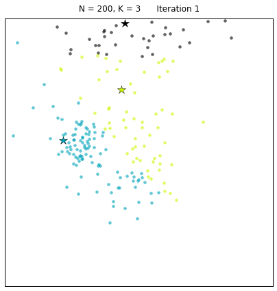
kmeans = KMeans(3, N=200)
kmeans.find_centers()
kmeans.plot_board()

The snippet above creates a board with 200 points around 3 clusters. The call to the find_centers() function runs the standard k-means algorithm initializing the centroids to 3 random points. Finally, the function plot_board() produces a plot of the data points as clustered by the algorithm, with the centroids marked as stars. In the image below we can see the results of running the algorithm twice. Due to the random initialization of the standard k-means, the correct solution is found some of the times (right panel) whereas in some cases a suboptimal end point is reached instead (left panel).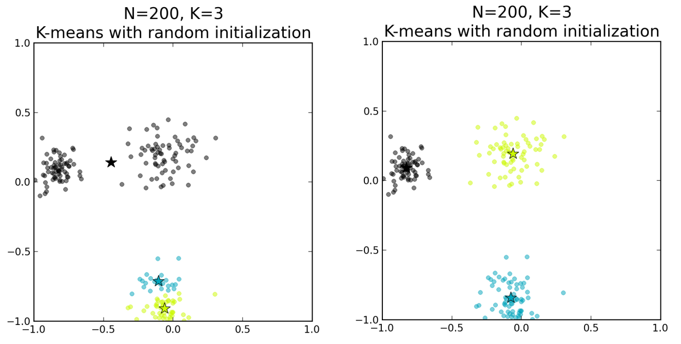

Let us now implement the k-means++ algorithm in its own class, which inherits from the class Kmeans defined above.

class KPlusPlus(KMeans):
    def _dist_from_centers(self):
        cent = self.mu
        X = self.X
        D2 = np.array([min([np.linalg.norm(x-c)**2 for c in cent]) for x in X])
        self.D2 = D2

    def _choose_next_center(self):
        self.probs = self.D2/self.D2.sum()
        self.cumprobs = self.probs.cumsum()
        r = random.random()
        ind = np.where(self.cumprobs >= r)[0][0]
        return(self.X[ind])

    def init_centers(self):
        self.mu = random.sample(self.X, 1)
        while len(self.mu) < self.K:
            self._dist_from_centers()
            self.mu.append(self._choose_next_center())

    def plot_init_centers(self):
        X = self.X
        fig = plt.figure(figsize=(5,5))
        plt.xlim(-1,1)
        plt.ylim(-1,1)
        plt.plot(zip(*X)[0], zip(*X)[1], '.', alpha=0.5)
        plt.plot(zip(*self.mu)[0], zip(*self.mu)[1], 'ro')
        plt.savefig('kpp_init_N%s_K%s.png' % (str(self.N),str(self.K)), \
                    bbox_inches='tight', dpi=200)

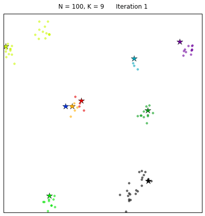
To run the k-means++ initialization stage using this class and visualize the centers found by the algorithm, we simply do:

kplusplus = KPlusPlus(5, N=200)
kplusplus.init_centers()
kplusplus.plot_init_centers()

Let us explore what the function init_centers() is actually doing: to begin with, a random point is chosen as first center from the X data points as random.sample(self.X, 1). Then, the successive centers are picked, stopping when we have K=5 of them. The procedure to choose the next most suitable center is coded up in the _choose_next_center() function. As we described above, the next center is drawn from a distribution given by the normalized distance vector $D_i^2 / \sum_j D_j^2$ . To implement such a probability distribution, we compute the cumulative probabilities for choosing each of the N points in X. These cumulative probabilities are partitions in the interval [0,1] with length equal to the probability of the corresponding point being chosen as a center, as explained in this stackoverflow thread. Therefore, by picking a random value $r \in [0,1]$ and finding the point corresponding to the segment of the partition where that $r$ value falls, we are effectively choosing a point drawn according to the desired probability distribution. On the right is a plot showing the results of the algorithm for 200 points and 5 clusters.

Finally let us compare the results of k-means with random initialization and k-means++ with proper seeding, using the following code snippets:

# Random initialization
kplusplus.find_centers()
kplusplus.plot_board()
# k-means++ initialization
kplusplus.find_centers(method='++')
kplusplus.plot_board()

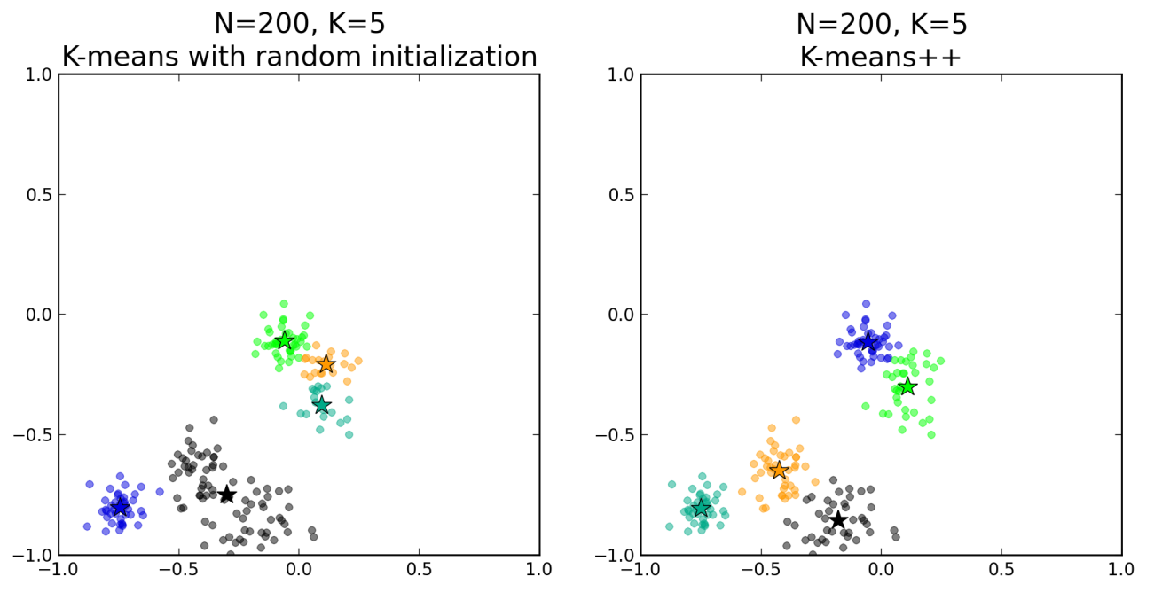
The standard algorithm with random initialization in a particular instantiation (left panel) fails at identifying the 5 optimal centroids for the clustering, whereas the k-means++ initialization (right panel) succeeds in doing so. By picking up a specific and not random set of centroids to initiate the clustering process, the k-means++ algorithm also reaches convergence faster, guaranteed by the theorems proved in the Arthur and Vassilvitskii article.

Table-top data experiment take-away message

The k-means++ method for finding a proper seeding for the choice of initial centroids yields considerable improvement over the standard Lloyd’s implementation of the k-means algorithm. The initial selection in k-means++ takes extra time and involves choosing centers in a successive order and drawing them from a particular probability distribution that has to be recomputed at each step. However, by doing so, the k-means part of the algorithm converges very quickly after this seeding and thus the whole procedure actually runs in a shorter computation time. The combination of the k-means++ initialization stage with the standard Lloyd’s algorithm, together with additional various techniques to find out an optimal value for the ideal number of clusters, poses a robust way to solve the complete problem of clustering data points.

December 27, 2013

Finding the K in K-Means Clustering

A couple of weeks ago, here at The Data Science Lab we showed how Lloyd’s algorithm can be used to cluster points using k-means with a simple python implementation. We also produced interesting visualizations of the Voronoi tessellation induced by the clustering. At the end of the post we hinted at some of the shortcomings of this clustering procedure. The basic k-means is an extremely simple and efficient algorithm. However, it assumes prior knowledge of the data in order to choose the appropriate K. Other disadvantages are the sensitivity of the final clusters to the selection of the initial centroids and the fact that the algorithm can produce empty clusters. In today’s post, and by popular request, we are going to have a look at the first question, namely how to find the appropriate K to use in the k-means clustering procedure.

Meaning and purpose of clustering, and the elbow method

Clustering consist of grouping objects in sets, such that objects within a cluster are as similar as possible, whereas objects from different clusters are as dissimilar as possible. Thus, the optimal clustering is somehow subjective and dependent on the characteristic used for determining similarities, as well as on the level of detail required from the partitions. For the purpose of our clustering experiment we use clusters derived from Gaussian distributions, i.e. globular in nature, and look only at the usual definition of Euclidean distance between points in a two-dimensional space to determine intra- and inter-cluster similarity.

The following measure represents the sum of intra-cluster distances between points in a given cluster $C_k$ containing $n_k$ points:

$\displaystyle D_k = \sum_{\mathrm{x}_i \in C_k} \sum_{\mathrm{x}_j \in C_k} ||\mathrm{x}_i - \mathrm{x}_j ||^2 = 2 n_k \sum_{\mathrm{x}_i \in C_k} ||\mathrm{x}_i - \mu_k ||^2$ .

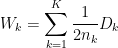
Adding the normalized intra-cluster sums of squares gives a measure of the compactness of our clustering:

$\displaystyle W_k = \sum_{k=1}^K \frac{1}{2n_k} D_k$ .

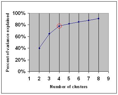
This variance quantity $W_k$ is the basis of a naive procedure to determine the optimal number of clusters: the elbow method.

If you graph the percentage of variance explained by the clusters against the number of clusters, the first clusters will add much information (explain a lot of variance), but at some point the marginal gain will drop, giving an angle in the graph. The number of clusters are chosen at this point, hence the “elbow criterion”.

But as Wikipedia promptly explains, this “elbow” cannot always be unambiguously identified. In this post we will show a more sophisticated method that provides a statistical procedure to formalize the “elbow” heuristic.

The gap statistic

The gap statistic was developed by Stanford researchers Tibshirani, Walther and Hastie in their 2001 paper. The idea behind their approach was to find a way to standardize the comparison of $\log W_k$ with a null reference distribution of the data, i.e. a distribution with no obvious clustering. Their estimate for the optimal number of clusters $K$ is the value for which $\log W_k$ falls the farthest below this reference curve. This information is contained in the following formula for the gap statistic:

$\displaystyle \mathrm{Gap}_n(k) = E_n^*\{\log W_k\} - \log W_k$ .

The reference datasets are in our case generated by sampling uniformly from the original dataset’s bounding box (see green box in the upper right plot of the figures below). To obtain the estimate $E_n^*\{\log W_k\}$ we compute the average of $B$ copies $\log W^*_k$ for $B=10$ , each of which is generated with a Monte Carlo sample from the reference distribution. Those $\log W^*_k$ from the $B$ Monte Carlo replicates exhibit a standard deviation $\mathrm{sd}(k)$ which, accounting for the simulation error, is turned into the quantity

$\displaystyle s_k = \sqrt{1+1/B}\,\mathrm{sd}(k)$ .

Finally, the optimal number of clusters $K$ is the smallest $k$ such that $\mathrm{Gap}(k) \geq \mathrm{Gap}(k+1) - s_{k+1}$ .

A Python implementation of the algorithm

The computation of the gap statistic involves the following steps (see original paper):

Cluster the observed data, varying the number of clusters from $k = 1, ..., k_{\mathrm{max}}$ , and compute the corresponding $W_k$ .
Generate $B$ reference data sets and cluster each of them with varying number of clusters $k = 1, ..., k_{\mathrm{max}}$ . Compute the estimated gap statistic $\mathrm{Gap}(k) = (1/B) \sum_{b=1}^B \log W^*_{kb} - \log W_k$ .
With $\bar{w} = (1/B) \sum_b \log W^*_{kb}$ , compute the standard deviation $\mathrm{sd}(k) = [(1/B) \sum_b (\log W^*_{kb} - \bar{w})^2]^{1/2}$ and define $\displaystyle s_k = \sqrt{1+1/B}\,\mathrm{sd}(k)$ .
Choose the number of clusters as the smallest $k$ such that $\mathrm{Gap}(k) \geq \mathrm{Gap}(k+1) - s_{k+1}$ .

Our python implementation makes use of the find_centers(X, K) function defined in this post. The quantity $W_k$ is computed as follows:

def Wk(mu, clusters):
    K = len(mu)
    return sum([np.linalg.norm(mu[i]-c)**2/(2*len(c)) \
               for i in range(K) for c in clusters[i]])

The gap statistic is implemented in the following code snapshot. Note that we use $B=10$ for the reference datasets and we span values of $K$ from 1 to 9.

def bounding_box(X):
    xmin, xmax = min(X,key=lambda a:a[0])[0], max(X,key=lambda a:a[0])[0]
    ymin, ymax = min(X,key=lambda a:a[1])[1], max(X,key=lambda a:a[1])[1]
    return (xmin,xmax), (ymin,ymax)

def gap_statistic(X):
    (xmin,xmax), (ymin,ymax) = bounding_box(X)
    # Dispersion for real distribution
    ks = range(1,10)
    Wks = zeros(len(ks))
    Wkbs = zeros(len(ks))
    sk = zeros(len(ks))
    for indk, k in enumerate(ks):
        mu, clusters = find_centers(X,k)
        Wks[indk] = np.log(Wk(mu, clusters))
        # Create B reference datasets
        B = 10
        BWkbs = zeros(B)
        for i in range(B):
            Xb = []
            for n in range(len(X)):
                Xb.append([random.uniform(xmin,xmax),
                          random.uniform(ymin,ymax)])
            Xb = np.array(Xb)
            mu, clusters = find_centers(Xb,k)
            BWkbs[i] = np.log(Wk(mu, clusters))
        Wkbs[indk] = sum(BWkbs)/B
        sk[indk] = np.sqrt(sum((BWkbs-Wkbs[indk])**2)/B)
    sk = sk*np.sqrt(1+1/B)
    return(ks, Wks, Wkbs, sk)

Finding the K

We shall now apply our algorithm to diverse distributions and see how it performs. Using the init_board_gauss(N, k) function defined in our previous post, we produce an ensemble of 200 data points normally distributed around 3 centers and run the gap statistic on them.

X = init_board_gauss(200,3)
ks, logWks, logWkbs, sk = gap_statistic(X)

The following plot gives an idea of what is happening:

The upper left plot shows the target distribution with 3 clusters. On the right is its bounding box and one Monte Carlo sample drawn from a uniform reference distribution within that rectangle. In the middle left we see the plot of $W_k$ that is used to determine $K$ with the elbow method. Indeed a knee-like feature is observed at $K=3$ , however the gap statistic is a better way of formalizing this phenomenon. On the right is the comparison of $\log W_k$ for the original and averaged reference distributions. Finally, the bottom plots show the gap quantity on the left, with a clear peak at the correct $K=3$ and the criteria for choosing it on the right. The correct $K$ is the smallest for which the quantity plotted in blue bars becomes positive. The optimal number is correctly guessed by the algorithm as $K=3$ .

Let us now have a look at another example with 400 points around 5 clusters:

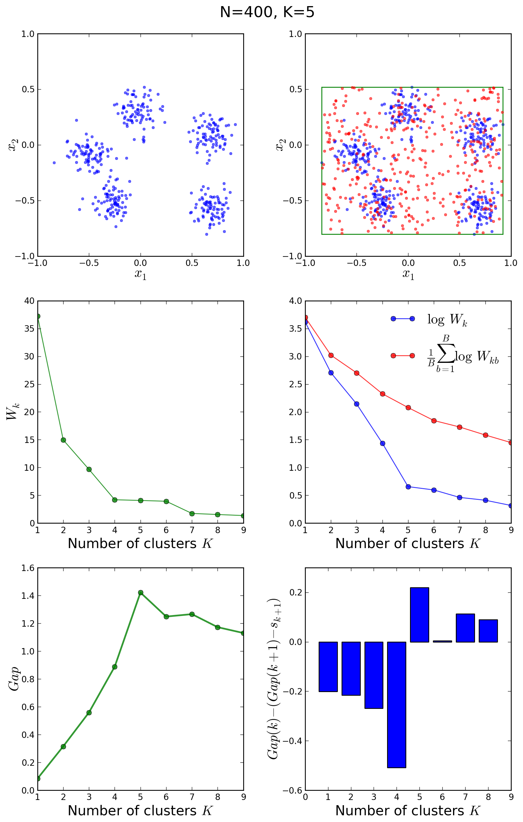
In this case, the elbow method would not have been conclusive, however the gap statistic correctly shows a peak in the gap at $K=5$ and the bar plot changes sign at the same correct value.

Similarly, we can study what happens when the data points are clustered around a single centroid:

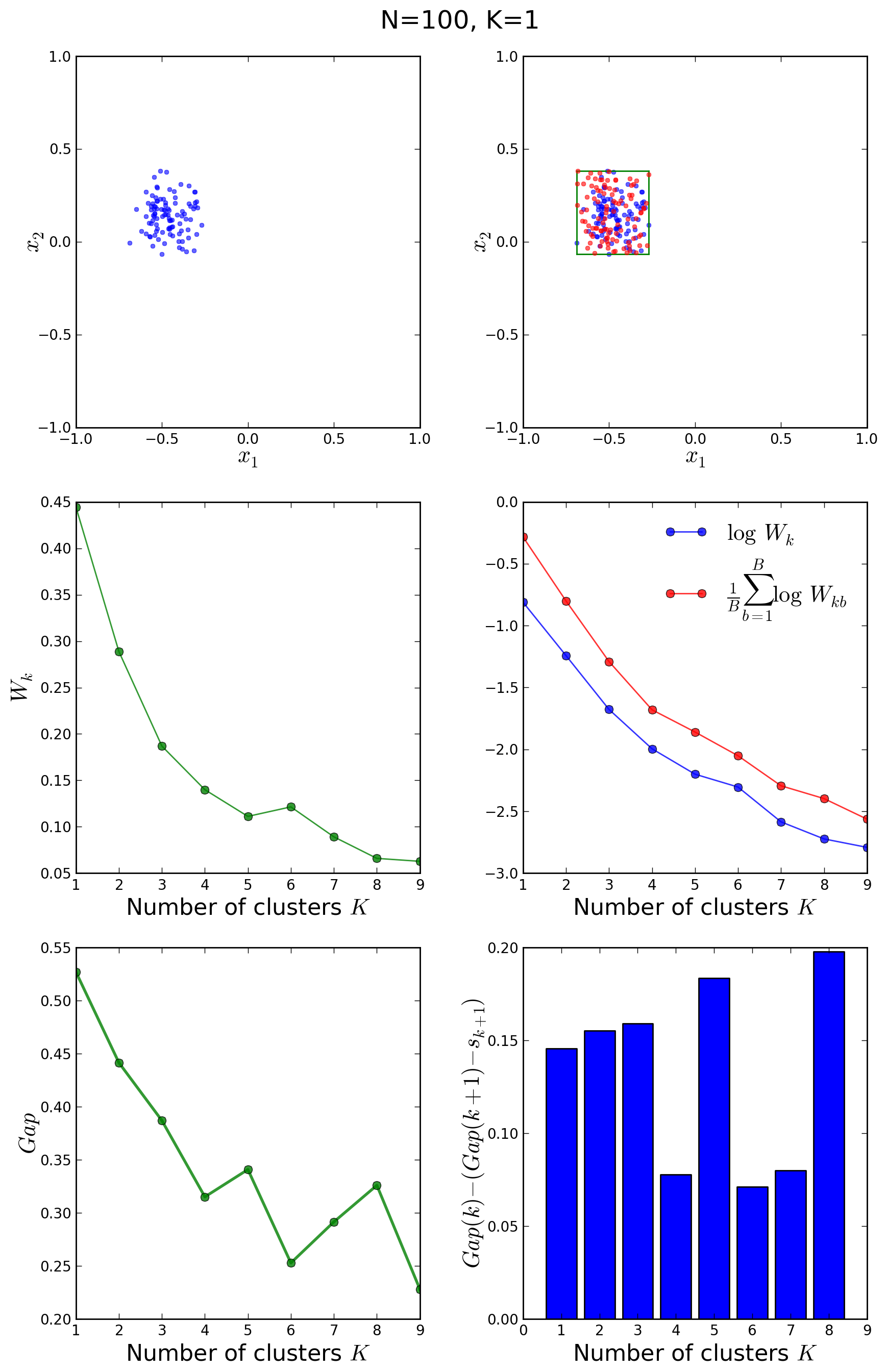
It is clear in the above figures that the original and the reference distributions in the middle right plot follow the same decay law, so that no abrupt fall-off of the blue curve with respect to the red one is observed at any $K$ . The bar plot shows positive values for the entire $K$ range. We conclude that $K=1$ is the correct clustering.

Finally, let us have a look at a uniform, non-clustered distribution of 200 points, generated with the init_board(N) function defined in our previous post:

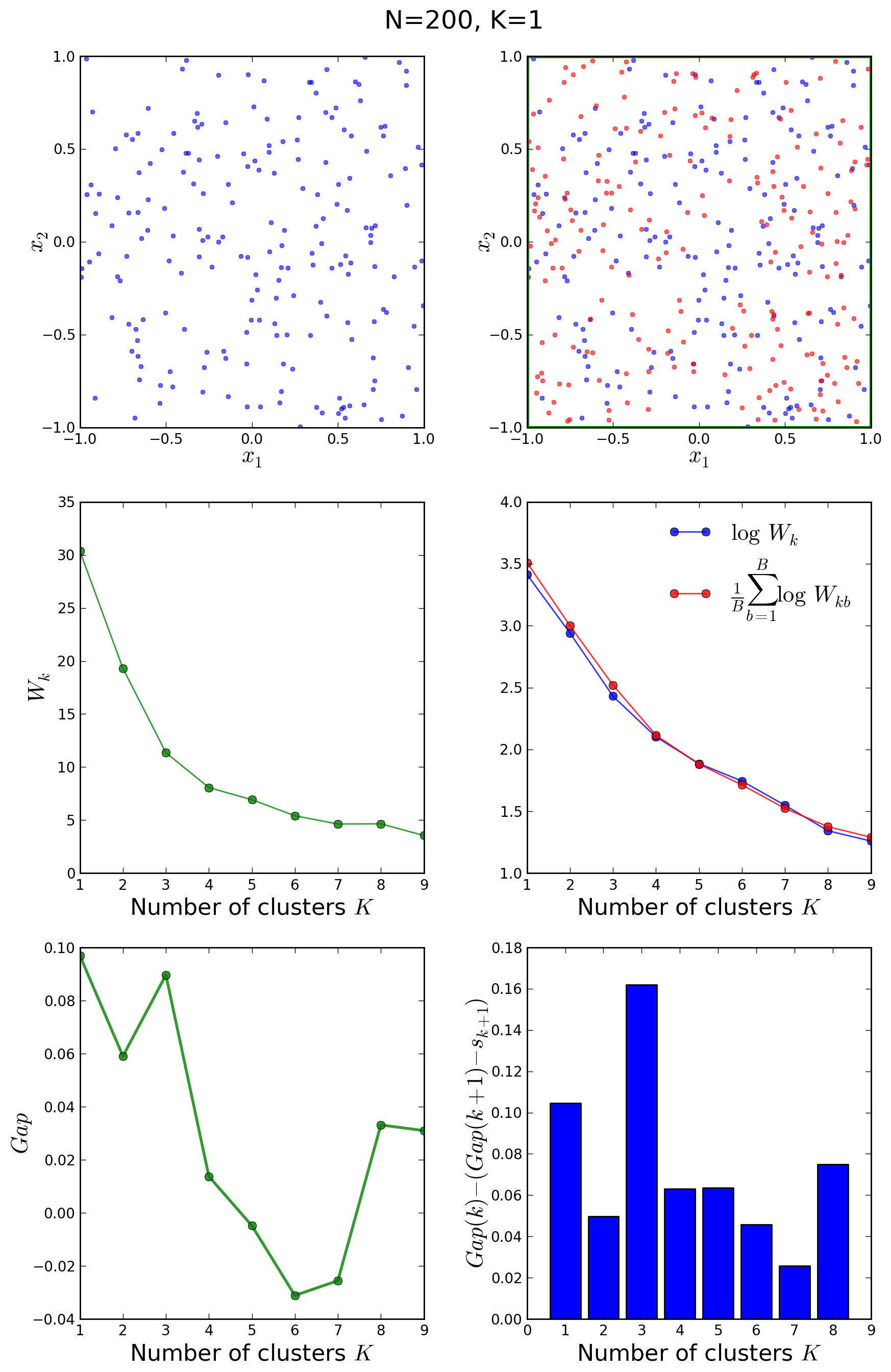
In this case, the algorithm also guesses $K=1$ correctly, and it is clear from the middle right plot that both the original and the reference distributions follow exactly the same decay law, since they are essentially different samples from the same uniform distribution on [-1,1] x [-1,1]. The gap curve on the bottom left oscillates between local maxima and minima, indicating certain structures within the original distribution originated by statistical fluctuations.

Table-top data experiment take-away message

The estimation of the optimal number of clusters within a set of data points is a very important problem, as most clustering algorithms need that parameter as input in order to group the data. Many methods have been proposed to find the proper $K$ , among which the “elbow” method offers a very clear and naive solution based on intra-cluster variance. The gap statistic, proposed by Tobshirani et al. formalizes this approach and offers an easy-to-implement algorithm that successfully finds the correct $K$ in the case of globular, Gaussian-distributed, mildly disjoint data distributions.

Update: For a proper initialization of the centroids at the start of the k-means algorithm, we implement the improved k-means++ seeding procedure.

Update: For a comparison of this approach with an alternative method for finding the K in k-means clustering, read this article.